Elvira Part 4 - Reinforcement Learning
Elvira Write-up Navigation Previous: Object Detection
Elvira uses an online Q-learning algorithm to make decisions based on the state space input received from the object detection pipeline. This post describes the reinforcement learning approach used, experimental setup, and discussion of the results.
Experiment Overview
Problem Formulation
Q-Learning Implementation
Results/Discussion
Q-Learning in Action
Experiment Overview
Colored discs are placed in the frame of Elvira’s camera. Elvira reacts autonomously based on the position of the colored discs and explores the state space with a goal of maximizing reward.
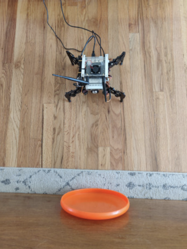
Top down view of the experimental setup
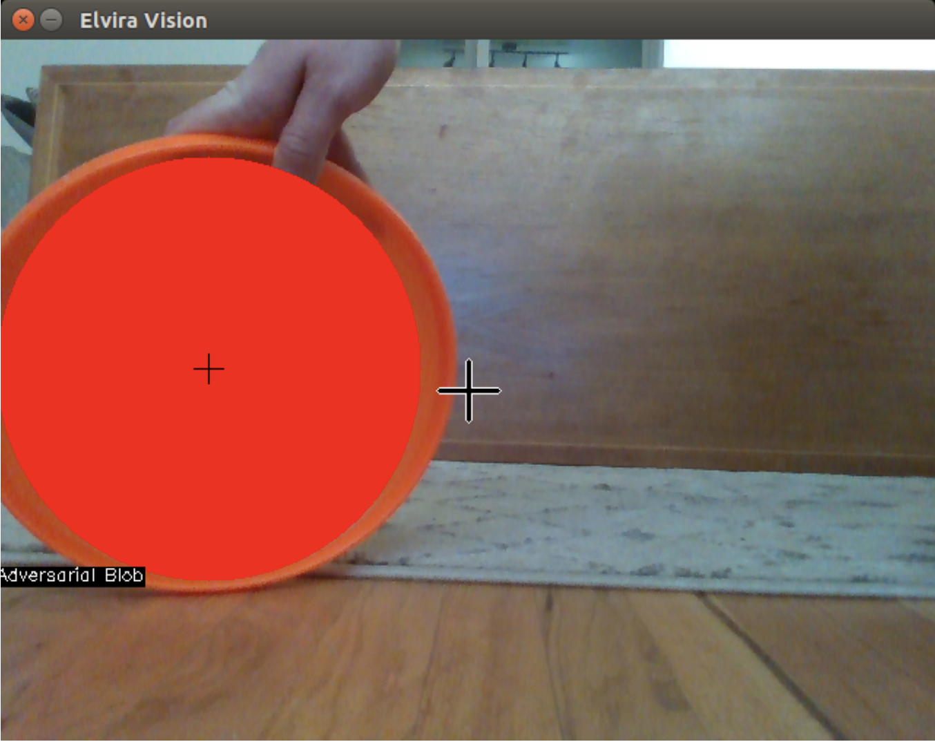
Camera frame which is extended into the state space - note the cross hairs at the center of the frame and the centroid of the detected blob
Problem Formulation
The problem is formulated as a Markov Decision Process according to the following 5-tuple \((S, A, T, \gamma, R )\), described in depth in the following sections:
\(S\): State Space
The state space is an n-dimensional tuple describing the proportion of image frame occupied by a blob.
The state space is generated in real-time from the RGB color feed coming from the camera. The object detection pipeline digests this RGB color feed and decomposes the blobs it detects into a “blobject” primitive. This primitive is defined as:
$$
\text{“blobject” } = [ i_{cm}, j_{cm}, N, radius, status]
$$
where:1 2
$$
\begin{align}
i_{cm} &= i \text{ centroid of detected blob (px)} \\
j_{cm} &= j \text{ centroid of detected blob (px)} \\
N &= \text{ Number of pixels in detected blob} \\
radius &= \text{ radius of selected blob (px)} \\
status &= \text{status of blob} \\
&\hspace{10pt} \text{ (“adversarial” vs “friendly”)}
\end{align}
$$
Each blob that is detected is maintained in a list and passed to the reinforcement learning pipeline.
Within this reinforcement learning pipeline the image frame is partitioned based on two user defined parameters: \(n_{bins}, dimsize\).
The following schematic gives a visual representation of the state space to aid in the following descriptions.
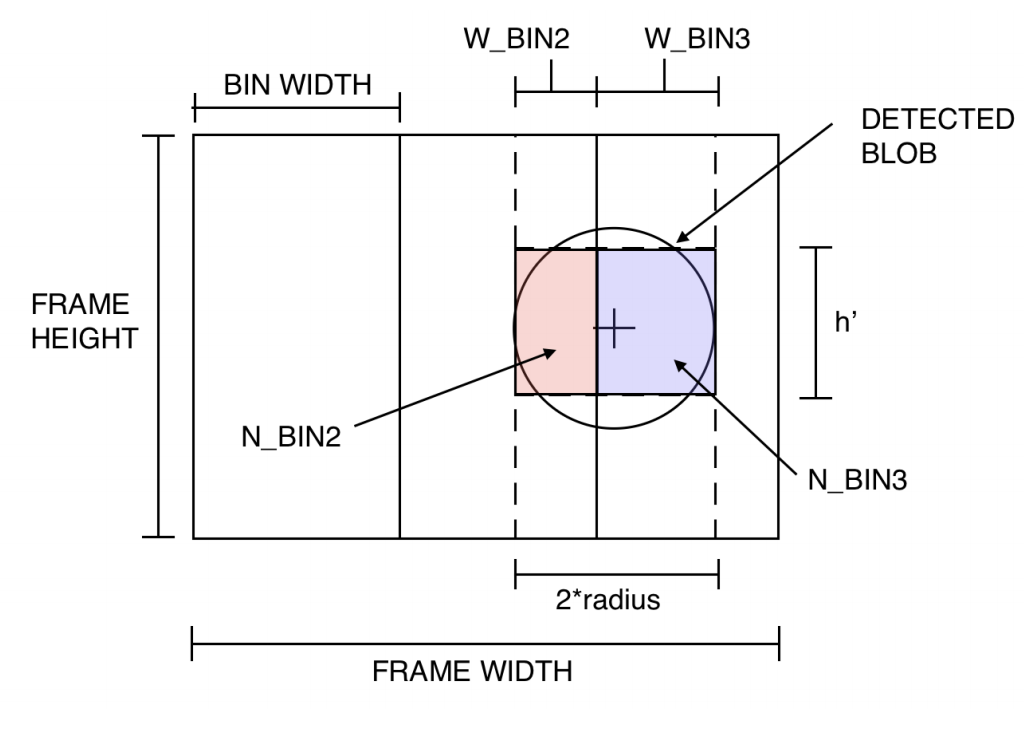
Blob state space; \(n_{bins} = 3\)
\(n_{bins}\) is the number of regions the image frame is horizontally partitioned into. For example, if \(n_{bins}=3\), the image frame would be divided into 3 parts.
\(dimsize\) is the interval resolution of each bin. Each partition can have a blob occupancy proportion \(\in [0,1]\). If the partition does not have any blob objects detected within its boundaries, its blob occupancy proportion \(=0\). If the entire image partition is filled with detected blob pixels, its blob occupancy proportion \(=1\). In order to make this more computationally tractable, we partition this blob occupancy proportion into intervals. If \(dimsize=3\), observed occupancy proportions would be grouped within some element of the following interval: $$ Interval = \big[(0, 0.33), (0.33,0.66), (0.66,1)\big] $$ Sticking with this example - if the image partition in question had a blob occupancy proportion \(=0.25\) it would be grouped into the interval \((0,0.33)\)
The blob occupancy proportion is determined based on the blob centroid and radius. Since the state space is based on horizontal image partitions, we cheat a little bit and represent the detected blob as a rectangle with width \(=2\times radius\) and a height \(h^`\).
$$ h^` = \frac{\pi\times radius^2}{2\times radius} $$
Using this simplified blob geometry, we can calculate the blob occupancy proportion \(N_{bin,i}\) with the following formula: $$ N_{bin,i} = \frac{W_{bin,i}\times h^`}{BinWidth\times FrameHeight}\in [0,1] $$
Finally, if you learn like myself, examples provide the most clarity: Using the example state space above, we note that one blob is detected in two image partitions. We see that \(N_{bin,2}=0.2, N_{bin,3}=0.4, n_{bins} = 3\), \(binsize=3\). This implies that any value \(N_{bin,i}\in [0, 0.33)\) would be grouped into the interval \([0, 0.33)\). This implies that for our example, the overall state space would be: $$ S_{example} = \big[(0,0.33), (0, 0.33), (0.33,0.667)\big] $$
Because of all the possible combinations of intervals and bins, the state space grows quickly with an increase in the user defined parameters. We can treat this like a combinatorics problem (ordered sampling with replacement) which implies that the state space can become quite large.
$$
\begin{align}
|S| = d^n, d&=dimsize \\
n &= n_{bins}
\end{align}
$$
\(A\): Action Space
The action space are the movements that Elvira can take: $$ A \in [CW, CCW, noRotate] $$ Where \(CW, CCW\) are \(45^{\circ}\) clockwise and counter-clockwise rotations and \(noRotate\) is an action where Elvira does not rotate.
\(T\): Transition Probabilities
The transition probabilities are deterministic in this formulation: any selected action will execute with probability = 1. Note that not all actions execute the same way due to servo tolerances and difficulties with quadruped motion patterns.
\(\gamma\): Discount Factor
A discount factor \(\gamma = 0.99\) was used.
\(R\): Reward Function
The reward function divides the state space into thirds and assigns rewards based on the contents of those regions:
- If there is an adversarial blob in the middle third of image frame (”scared zone”), the actor gets a negative reward.
- If there are no blobs detected or an adversarial blob is detected but outside of the middle third (out of frame or in the ”safe-zone”), the actor gets a positive reward.
- If the actor chooses a movement action (any action besides \(noRotate\)) it gets an additional negative reward penalty.
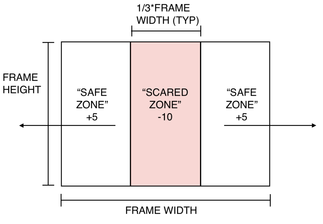
Reward function schematic
Q-Learning Implementation
Elvira uses an unmodified implementation of the Q-learning algorithm 3 using a modified \(\epsilon\)-greedy function for policy selection. The algorithm is described below4:
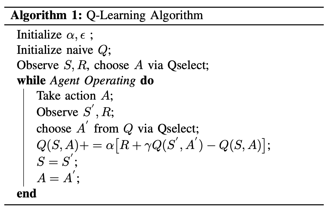
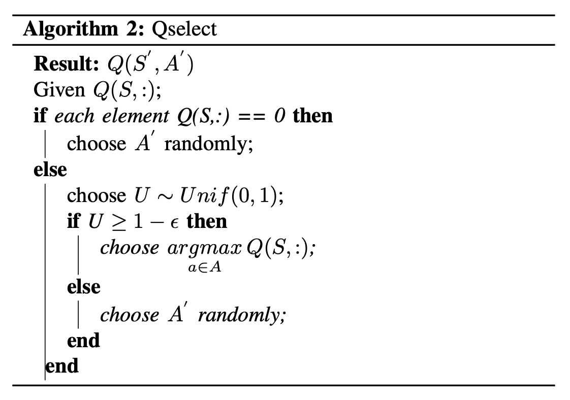
The policy selection algorithm “Qselect” is a modified implementation of \(\epsilon\)-greedy; if the algorithm encounters a \(Q(S,:)\) region of the state space it has not explored (aka the expected reward for all actions is totally naive), it will randomly select an action by drawing from a uniform distribution.
Based on the descriptions of the state and action spaces above, the size of \(Q\) is: $$ |Q| = |A|\times|S| = |A|\times d^n $$
Results/Discussion
Overall the experiment produced desirable results with a lot of room for improvement. Several different reward functions were used before finally settling on one that would cause the agent to converge to an optimal terminal state (not moving and not observing and ”adversarial” blobs). The different reward functions tested are shown in the following table.
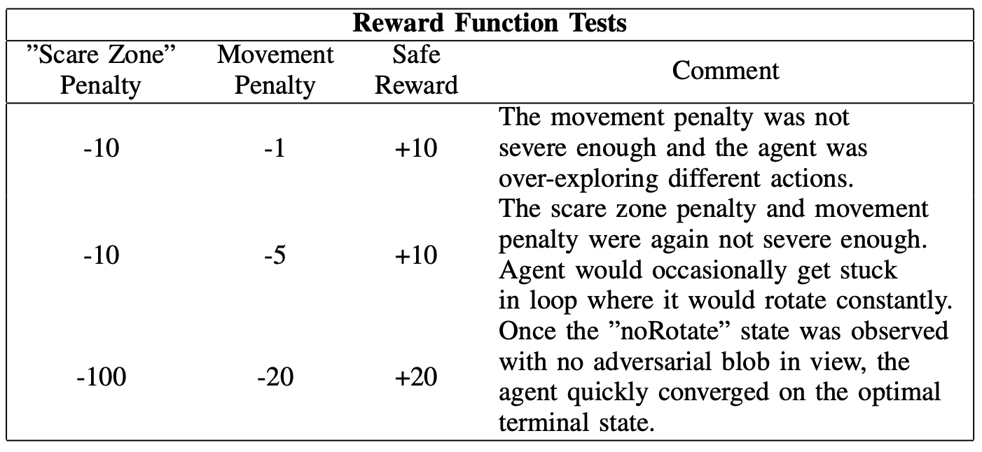
Eventually the reward function described in the third row of the table was used. The rewards were weighted appropriately so that it was penalized enough for observing a ”scary” state space. Once it found the \(noRotate\)/safe area portions of the state space it quickly converged into a terminal state.
The following plot shows the sum of the rewards over time; different colored lines represent different agent training epochs. As noted previously, all training epochs end with a linearly increasing sum of rewards by the end of the training epoch. This implies that in all cases the agent was able to find the optimal terminal condition. There is a large amount of variation in how long it took for the agent to find this optimal terminal condition which is a product of the naive \(\epsilon\)-greedy policy selection at the start of each epoch.
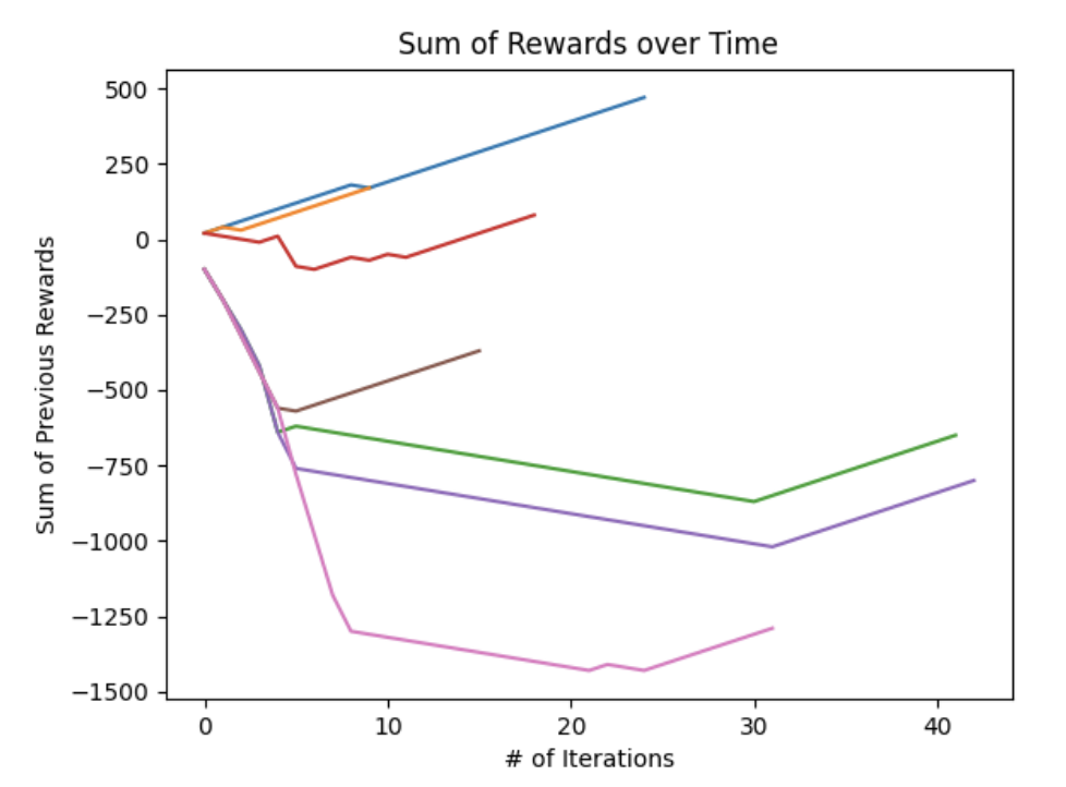
In cases like the orange and blue training epochs, actions that quickly led to escaping the negative reward space allowed for quick convergence (For example, the orange and blue lines immediately selected \(noRotate\) based on a lucky -greedy happenstance). Conversely, training epochs like the pink and purple lines took substantially more training iterations before reaching the optimal terminal state.
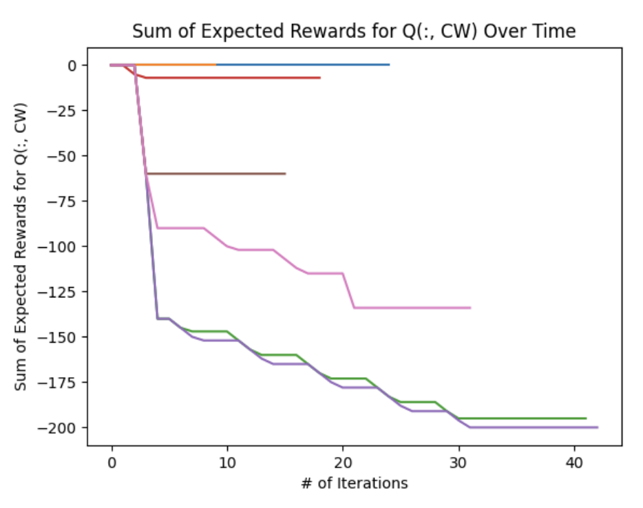
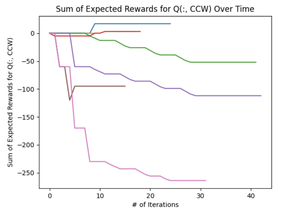
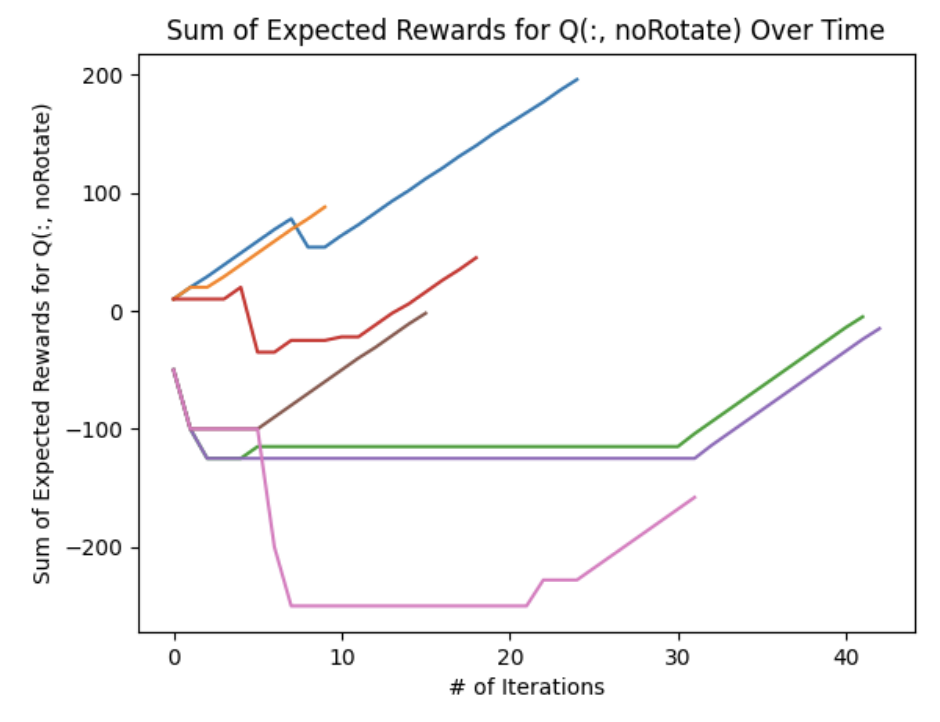
The following figures show the sum of the expected rewards across the entire \(Q\) matrix for each action. We notice two prominent trends: there was a consistent continuously decrease in expected rewards during each \(CW, CCW\) iteration whereas the \(noRotate\) plot generally shows an increasing expected reward during each iteration. This implies that as the agent explores the state space, it eventually discovers that the \(noRotate\) action will yield a higher expected reward than the \(CW\) and \(CCW\) actions.
Some errant behavior was observed, especially during the reward function testing. Occasionally the actor would get into a state where it would continuously spin in circles by perpetually choosing a \(CW\) or \(CCW\) action. This was likely due to a movement penalty that was too small and the fact that the initial action chose may have been the \(noRotate\) command which would have given a negative reward - the starting condition had an ”adversarial blob” occupying the middle third of the screen.
Reflections
Overall I am pleased with how this project turned out given the complexity of implementing online reinforcement learning (RL) on hardware.
Hardware I think I greatly underestimated how much complexity was introduced by implementing RL on hardware. I think this will probably be the last time I ever work with a robot with legs because implementing walking was such a monumental pain in the ass. This was also a great avenue to learn ROS, however I also faced some major issues with the ROS/Julia callback functions which resulted in me using print statements as my only debugging tool. I think this generally distracted from the core of the project which should have been implementing a more robust RL algorithm. I think that because I spent so much time on the hardware side of things, my actual experimental setup was very simple and imperfect - future RL pursuits will probably be simulation only unless I have a lot more time.
Algorithm Selection I think that this project demonstrated that Q-Learning is probably not the best algorithm for online learning. I am not confident that Elvira was fully exploring the entire state space and her behavior was sometimes inconsistent and erratic. I think a lot of this was due to the difficulties I had in implementing a reliable walking functionality; sometimes the CW, CCW commands yielded inconsistent motion which in turn yielded inconsistent rewards. Hardware issues aside, Q-Learning is not the most complex algorithm. I think the approach is intuitive and foundational, however future simulation RL pursuits will focus on implementing something more bleeding edge.
- Note that the origin of the image is in the upper left hand corner of the image frame. This is typical in image processing but inconsistent with how many people (myself included) typically visualize the origin of a plot (aka lower left hand corner). [return]
- The (status) component is unused in this implementation; future implementations may introduce disks wherein a positive reward is conferred for “looking” at friendly blobs. [return]
- Watkins, C.J.C.H., Dayan, P. Q-learning. Mach Learn 8, 279–292 (1992). https://doi.org/10.1007/BF00992698 [return]
- Richard S. Sutton and Andrew G. Barto. 2018. Reinforcement Learning: An Introduction. A Bradford Book, Cambridge, MA, USA. [return]