Beer Vision
I like beer, probability, and computer vision. This is a little toy project I put together that attempts to quantify the emission rate of bubbles when you pour a glass of beer. I’m using Julia and Upslope Citra Pale Ale. Github repo can be found here.
Image Processing
Finding a Distribution
Approximating the Exponential
Discussion
Image Processing
We begin by creating a gif by stacking all the images into a 3D array (2D images with a 3rd dimension representing time). Then we execute the following image processing pipeline:
Background Subtraction
First, we convert the colored image array to grayscale and take the average over all frames to create a threshold baseline for each frame. By taking the average across all frames, the static portions of the image are preserved but the moving portions disappear (or become streaks in practice). We compare this to individual frames to isolate out the moving portions of the image.
Below is a comparison of a video frame and the mean average background baseline image; note that the bubbles have largely disappeared:
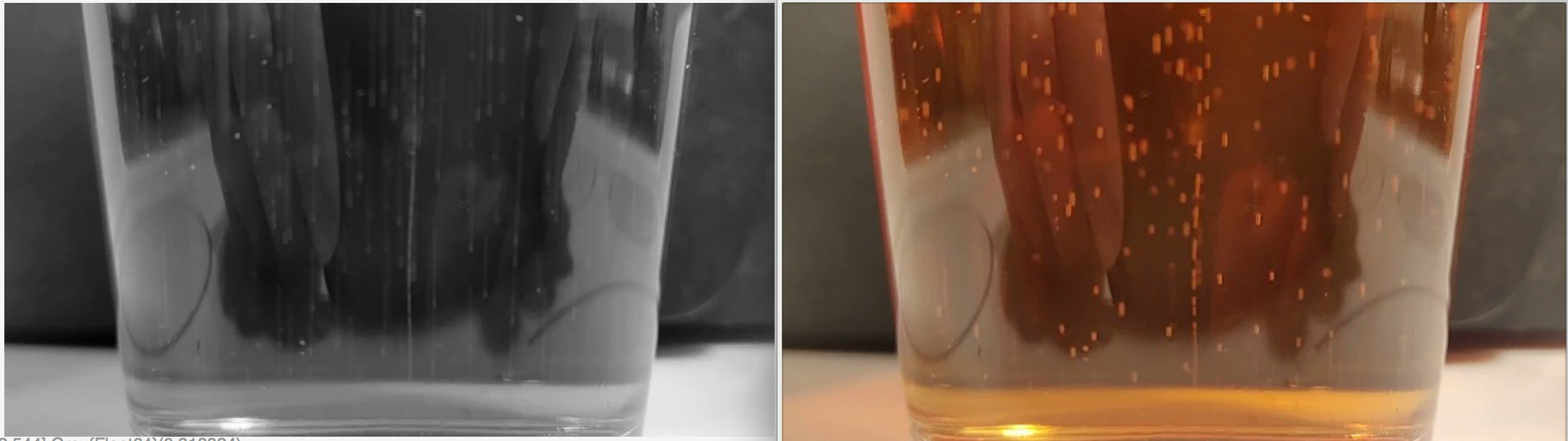
Baseline image (grayscale) vs video frame (color)
You can see that this gives a pretty good baseline of the static portions of the image. You can also see that there is some light streaking which is a product of the bubbles moving in straight lines. I think a higher frame rate video would help get a cleaner baseline.
Now that we have a ground truth we can “subtract” the baseline image from the video frames. If the percent difference of two pixels is greater than a user defined threshold (I’m using ~0.25) we turn that pixel white. Anything smaller we turn black. When we do this to all the frames in the video we generate the following binary mask:
“Bubbles Noire”
Centroid Detection Algorithm
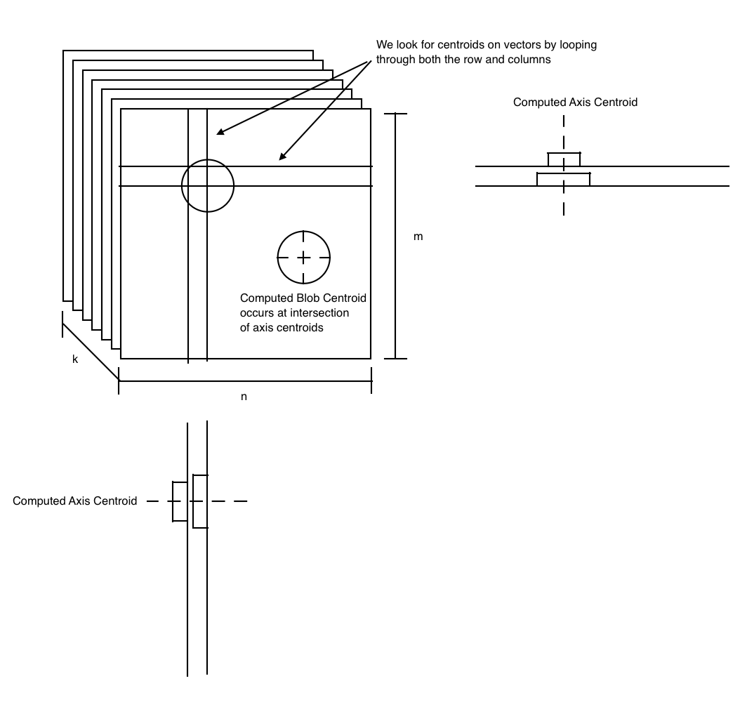
My bubble centroid detection algorithm doesn’t actually locate any blobs, it just computes the centroid for any thresholded binary mask object in two directions then looks for the intersection. The pseudocode and associated diagrams below explain how the algorithm works:
Pseudocode
|
|
Description of Algorithm
As shown in the pseudocode section, we see that we loop through both the columns and rows to determine the centroid of blobs in both axes. An offset of one pixel in the thresholded image (black vs white) will delineate between blobs. We don’t actually have any knowledge of what the size or shape of the blob is, just the lines drawn through the two centroidal axes. We find the centroid of the blob at the intersection of these two lines. A visual aid is provided below to help describe what the algorithm is doing.
When run, it produces the image below. Notice that the thresholded binary mask objects have been replaced with small (and sometimes non-orthogonal) crosses at the centroid of the detected objects.
Performance
Obviously this is a pretty inefficient algorithm - O(m*n*k) due to all the nested for loops. Luckily Julia comes to the rescue and we don’t suffer too much performance wise. Running on my 2012 MBP (ancient!) I got the following rough benchmarks. (Overall time doesn’t include any probability estimation stuff).
| # Frames | Overall Time | Centroid Algorithm Time |
|---|---|---|
| 10 | 11s | <1s |
| 100 | 88s | 3s |
| 200 | 181s | 7s |
Finding a Distribution
Now that we have a numerical representation of the centroids of the bubbles, we can begin to estimate the bubble distribution. The experimental setup is shown in the following figure:
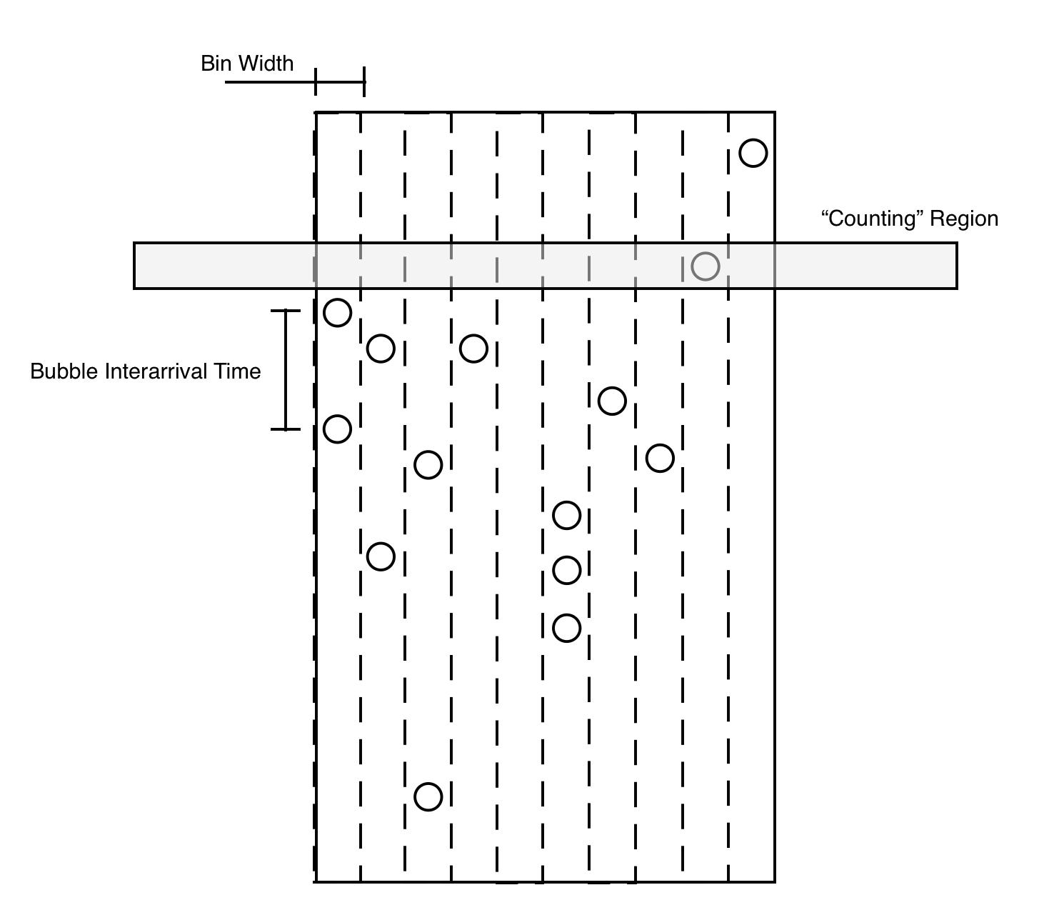
Experimental Diagram of Beer in Cup
The cup will be divided into several bins. We know that bubbles tend to only rise upwards and we ignore the possibility of a bubble moving laterally from its emission point. As bubbles rise up, they will pass through the “counting region” which will increment a counter for the bin and record the frame number of the hit. From this we can back out the bubble interarrival time based on the computed video frame rate (reference the appendix if you’re curious how this is computed).
The resulting output overlaid with the diagram stuff is shown below:
Behind the scenes the program is counting every time the centroid intersection occurs in the counting region (visually shown by the transition from purple to green). This increments up the bin counter and records the interarrival time since the previous hit. It then resets the timing counter for that bin and the process restarts. After the whole video is analyzed, we generate a histogram similar to the following plot. Note that I truncated off the bin for interarrival times in the first bin (0-0.03s for for a 30fps video) - I’ll discuss this in the next section.
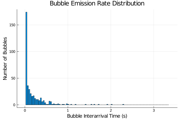
As you can see we have something that appears to resemble an exponentially distributed random variable. Now let’s see if we can characterize the rate parameter.
Approximating the Exponential
My first attempt to approximate the exponential was using the “method of moments” which is basically just a fancy way to say that I took the sum of all the interarrival times that were recorded and divided that by the total number of hits. More rigorously, I estimated the rate parameter such that:
Let \(X_i\) be experimentally collected bubble interarrival times. Let \( n \) be the number of samples collected.
$$
E[{\hat{X}}] = \frac{1}{n}\sum X_i
$$
$$
\bar{\lambda}=\frac{1}{E[\hat{X}]}
$$
As mentioned in the previous section, I truncated off the first bin of data because I had a ton of consecutive hits between frames. I talk about this more in the discussion section but the short version is that I think my interarrival time collection is not accurate - as I result I had a ton of bubble counts in consecutive frames. If we were to plot the histogram without truncation and a computed rate using the non-truncated data, it would look like:
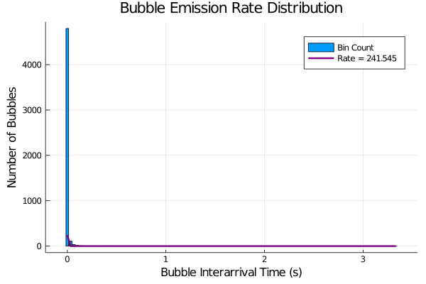
Plot without no truncation and method of moments rate calculation
This is not very pretty looking which is a big reason why I decided just to toss out data from the first bin. Even with this, we still see that the method of moments is giving us a bad rate parameter:
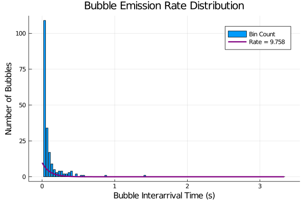
Plot with truncation and method of moments approximation
At this point, I don’t buy that my data collection pipeline is working all that well; however I still think that I can approximate the distribution that has formed with the data that I collected. I chatted about this with one of my probability professors who recommended I formulate it like an optimization problem: minimize error between my experimental distribution and an exponential with an optimized rate parameter. More formally, this looks like:
Let \(\hat{p}\) be the probability of some \(X_{i,b}\) occurring in some interval (bin) \(b \in [t, t+s]\). Let \(n_{b}\) be the number of \(X_{i,b}\in b\). Let \(A = \{\lambda_1, \lambda_2,…\}\) where \(\lambda_a \in A\) is the rate parameter for an exponential distribuion. Let \(p\) be the probability of some event occuring within \([t, t+s]\) for some \(exp(rate=\lambda_a)\).
$$ p = \int_b \lambda_a e^{-\lambda_a x}dx $$ $$ \hat{p} = \frac{1}{n_b}\sum X_{i,b} $$ $$ \bar{\lambda} = \underset{\lambda_a \in A}{argmin}\sqrt{\sum (\hat{p}-p)^2} $$
In less math-ey terms, I used the pdf of an exponential with a range of different rate parameters to compute probability bounded by the bin intervals (area under the curve between bins). I then compared this to the empirically collected “bin areas” from my bubble detection pipeline. By trying different rate parameters, I was able to see which rate parameter would cause the smallest error between the optimized exponential distributions and my collected data.
I used the trapezoidal rule for my numerical integration. When I evaluated this, I ended up computing a rate parameter of about 20. I generated several plots to help visualize/evaluate this computed rate parameter.
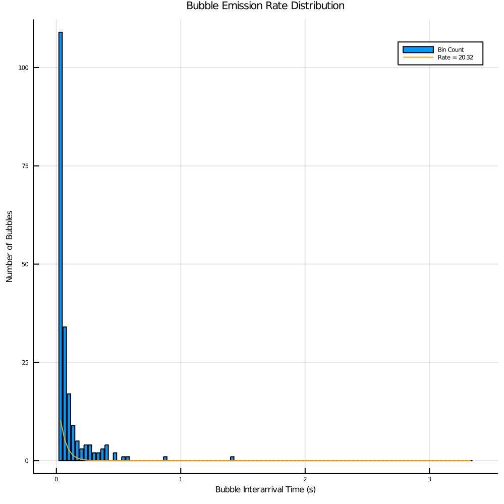
- Histogram
This first plot is of an exponential distribution based on the computed rate compared to the histogram. As you can see, I think that this was a better characterization of the histograms exponential distribution. (Note the differences in scale are a bit misleading but convey general trend information).
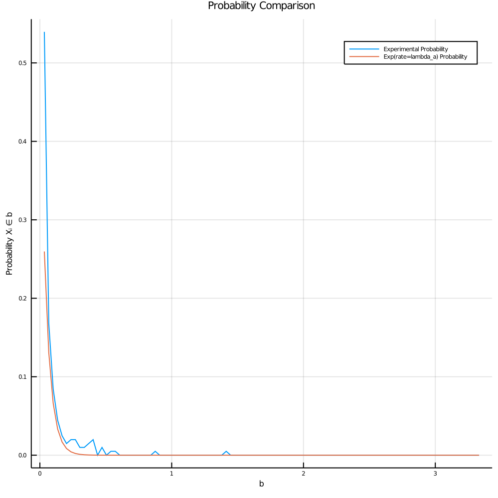
- Probability Comparisons
This next plot is of an exponential distribution with the calculated rate plotted against the empirical probabilities (# events in bin/total number of events). The curves appear to be a better approximation for shorter interarrival times in the distribution but fall apart for some of the middle interarrival times. These small interarrival terms have larger probabilities and thus carry more weight in the optimization function which explains why we see the deviation.
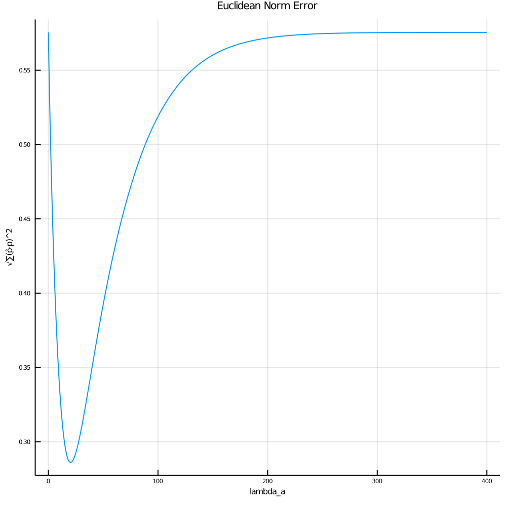
- Optimization Error
The final plot is the error calculated as I tested all possible rates in the set {A}. We see that we minimize error at a rate of around 20 as reported in the histogram plot.
Discussion/Future Exploration
I think there are several weak points to my approach that I’d like to mention:
Because my counting process is just looking for the centroid intersection of a bubble, it doesn’t necessarily track if that intersection has been counted in previous frames. To combat this, I tried to use a small counting window, however this also runs the risk of having a centroid intersection “jump over” the counting window between frames if moving quickly enough. I think the best solution to this problem would be to use a higher frame rate video.
I think that bin width also matters as well - as you can see in the video above some bins have streams of bubbles from different emission points that are being counted together. I think that there might be some argument to be made in terms of thinning or superimposing the underlying Poisson process that governs the emission rate, however I think the easiest thing to do would just have thinner bin widths.
There are several future areas that I would like to explore now that I have this pipeline in place. A super neat one would be to look at how different types of beers (eg stout vs lager) might impact the emission rate. Correlations could be drawn between beer specific gravity, etc. Additionally, it would be interesting to look at data from a longer time frame (eg bubble data every ten minutes for an hour) to quantify the bubbles as a non-homogenous Poisson distribution with a time variant rate parameter.
Appendix: Extracting Frame Rate
One thing I realized early on in making this post is that if I want to quantify this as a rate, I need accurate timing data. Eventually I should probably capture video with a time stamp on it, however in the meantime, I just changed my extractframes() code to write frames until it exited with an error:
|
|
|
|
Given that I generated 230 frames in 7.85s, about 29.3 frames per second. According to my camera manufacturer the OnePlus 6t can shoot at 1080p 30/60fps. the outputted resolution for the test video bubbles1.mp4 is 1920x1980 so we can confidently say that this video is 1080p/30fps.
This has some real implications for the accuracy of my rate so I wasn’t sure if I should use the 30fps number or the 29.3fps number. Because I was not super confident in my (potentially hacky) way of splicing frames, I decided to assume that the 29.3fps number is a more accurate number (the frame splice may not have occurred at each frame exactly). This is confirmed by looking at another video bubbles2.mp4 which is 5.53 seconds long and generates 162 frames which gives an actual frame rate of 29.3fps as well.
Upon some additional research I realized that ffmpeg gives you video on frame rate as well. By running, you can get the following output.
|
|
bubbles1.mp4 we see that we get 7.85 seconds with an actual fps = 29.71 which is about a 1.4% difference compared to the calculated fps of 29.3fps. This is a pretty minimal difference so I’m going to use the ffmpeg output in the calculations. This avoids us having to generate all the possible frames until the program errors out.
I was having some real issues with all the Julia pipeline stuff for accessing the shell so I just ended up writing it to a text file that I read using the following code:
|
|